Research Article - Biomedical Research (2018) Volume 29, Issue 10
Histopathological breast-image classification with restricted Boltzmann machine along with backpropagation
Abdullah-Al Nahid*, Aaron Mikaelian and Yinan Kong
School of Engineering, Macquarie University, Sydney, Australia
- *Corresponding Author:
- Abdullah-Al Nahid
School of Engineering
Macquarie University
Sydney, Australia
Accepted date: March 29, 2018
DOI: 10.4066/biomedicalresearch.29-17-3903
Visit for more related articles at Biomedical ResearchAbstract
Deaths due to cancer have increased rapidly in recent years. Among all the cancer diseases, breast cancer causes many deaths in women. A digital medical photography technique has been used for the detection of breast cancer by physicians and doctors, however, they need to give more attention and spend more time to reliably detect the cancer information from the images. Doctors are heavily reliant upon Computer Aided Diagnosis (CAD) for cancer detection and monitoring of cancer. Because of the dependence on CAD for cancer diagnosis, researchers always pay extra attention to designing an automatic CAD system for the identification and monitoring of cancer. Various methods have been used for the breast-cancer image-classification task, however, state-of-the-art deep learning techniques have been utilised for cancer image classification with success due to its self-learning and hierarchical featureextraction ability. In this paper we have developed a Deep Neural Network (DNN) model utilising a restricted Boltzmann machine with “scaled conjugate gradient” backpropagation to classify a set of Histopathological breast-cancer images. Our experiments have been conducted on the Histopathological images collected from the BreakHis dataset.
Keywords
Accuracy, Classification, Deep neural network, Restricted Boltzmann machine, Tamura
Introduction
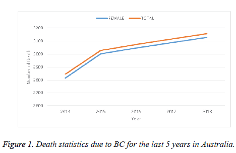
Many patients in the world suffer from cancer. There are different kinds of cancer, among them Breast Cancer (BC) is a prominent one, and is specifically a serious health threat to women. As a case study, Figure 1 shows the death statistics due to BC in Australia for the last 5 years. This figure shows that the death trend due to BC increased every year at an alarming rate in Australia. This might be considered as an example of the BC situation throughout the world. Obviously this causes a serious human and social impact. Proper and timely detection of BC can save or at least improve the condition of susceptible people. Along with other conditions, the detection of BC largely depends on investigation of biomedical images captured by different imaging techniques such as X-Rays, mammogram, magnetic resonance, histopathological images, etc. For perfect diagnosis of BC, a biopsy can produce reliable results with confidence. Histopathological images are used as a standard image for cancer diagnosis. However, their analysis is very time-consuming and needs extra attention for the perfect diagnosis along with the expertise of the physicians and doctors.
The history of using machine-learning techniques for general image classification is a long one. Using the advancement and the deliverable engineering of image classification, scientists have used such techniques for medical image classification. An important part of the image classification is appropriate selection of features such as the Gray-Level Co-occurrence Matrix (GLCM), Tamura, etc. as well as classifier models such as Support Vector Machine (SVM), Random Tree (RT), Random Forest (RF), etc. [1]. In a few cancer imageclassification cases, scientists also extract information on nuclei. Diz et al. utilised both GLCM and Gray-Level Run Length Matrix (GLRLM) for mammogram image (400 images) classification and achieved 76.00% accuracy [2] where they employed the RF algorithm. The RF algorithm has also been used for histopathological image classification. Zhang et al. [3], Bruno et al. [4], and Paul et al. [5] utilised histopathological images with different features. Paul et al. [5] utilised the Harlick features, Bruno et al. [4] used the curvelet transform and Local Binary Pattern (LBP), Zhang et al. [3] implemented the curvelet transform, GLCM and CLBP together for classification.
The SVM is another popular and useful classifier for image classification. For the very first time Bazzani et al. utilised SVM techniques for breast image classification. Martins et al. [6] utilised Ripleys Function along with an SVM for Mammogram image classification and obtained accuracy, sensitivity and specificity of 94.94%, 92.86% and 93.33%, respectively.. Chang et al. [7] utilised an auto-correlation coefficient for ultrasound breast-image classification and obtained 85.6% accuracy. Kavitha et al. [8] implemented histogram, textural (using the Gabor Filter) features and a few clinical features which were extracted from the images. They also resorted to SVM techniques for the image classification and obtained 90% Accuracy. Chang et al. classified a set of tomography images (250 images) using SVM techniques where the images are surrounded by speckle noise [9]. Fractional Fourier Transform (FFT) information has been used as features by Zhang et al. [10] for Mammogram image classification using SVM along with Principal Component Analysis (PCA) techniques. Dheba et al. [11] utilised Laws texture features to classify images into Benign and Malignant (MIAS database) and achieved 86.10% accuracy. They performed their experiment on 200 images and obtained 92.16 ± 3.60% accuracy. It is found that the kernel method along with the SVM technique can improve the classifier performance. Naga et al. [12] classified the Micro-calcification clusters in Mammogram images using Gaussian and polynomial kernels.
Along with other classifier techniques NN techniques have always been a strong tool for image classification. In 1991 Dawson et al. utilised an NN for a BC image classifier [13]. Literature shows that, the neural network technique has been very successful for the analysis and classification of images. Recently, the Deep Neural Network (DNN) technique has emerged as a popular method for the analysis of images for the classification task, following the famous model AlexNet proposed by Krizhevsky et al. [14]. They proposed their techniques for the image-classification issues [14] based on a Convolutional Neural Network (CNN), a branch of DNN. After the work of Alex, advanced engineering of this technique has been used for various image-classification tasks. Hai et al. proposed a fast-scanning Deep Neural Network (fCNN) method for the image-classification task [15], where they utilised seven convolutional layers for analysis of the images. Wu et al. [16] used CNN for global feature-extraction for mammogram (40 images) image classification and achieved a sensitivity of 75.00% and specificity 75.00%. Mammographic breast-density classification was done using HT-L3 convolution by Fonseca et al. [17]. Rezaeilouyeh et al. [18] implemented both local and global features and utilised CNN for histopathological image classification. They utilised the shearlet transform for extracting local features and achieved a best accuracy of 86 ± 3.00%. Xu et al. [19] utilised the DCNNN-cut- SVM methods together for Histopathological breast-image classification and obtained an ROC of 93.16%. For Nuclease detection, the spatially constrained CNN was employed by Sirinkunwattana et al. [20]. Huynh et al. combined transfer learning and ensemble techniques for Mammographic image classification. Kooi et al. [21] resorted to global crafted features along with the Transfer learning method (VGG model) for Mammographic image classification.
The Deep Belief Network (DBN) is another branch of DNN which is a recent concept, proposed by Hinton et al. in 2006 [22]. For the first time they used Restricted Boltzmann Machine (RBM) techniques for Modified National Institute of Standards and Technology (MNIST) character recognition. Discriminative Deep Belief Networks (DDBN) were proposed by Yan Liu et al. for visual data classification and they utilised backpropagation techniques [23]. Ahmed et al. preferred the DBN method for the breast-cancer classification task [24]. For their analysis, they used the Wisconsin breast cancer data set, which gives nine features for each image. So, instead of directly working on the images, the authors used the available features and DBN techniques with backpropagation.
The literature shows that a few studies have been performed on histopathological breast image classification using Tamura features. Most of the work has been conducted on well-known datasets like MIAS and DDSM along with some histopathological images. Fabio et al. provide a new set of histopathological breast images in the BreakHis dataset and they did BC image classification using a few dierent classifiers doing image classification largely relies on how we select the features for the classification task. In this paper we have classified histopathological (BreakHis) breast images using Tamura features and RBM along with contrast corrections. The overall architecture of this paper is organised as follows: Section 1 gives a brief description concerning the breast-image classification issues; Section 2 image-classification model; Section 3 describes the proposed RBM model for the classification; Section 4 describes the contrast correction algorithms in a brief; Section 5 describes the feature-extraction methodology; Section 6 describes and analyses the results; and Section 7 concludes the paper.
Image-Classification Model
Successful image classification depends on a number of steps such as image pre-processing, feature-extraction and using image-classifier tools. Depending on the image pre-processing steps we have proposed two algorithms:
• Algorithm-1: This algorithm does not apply any preprocessing steps before feature-extraction. Algorithm 1 directly extracts Tamura features from each image, and the features are fed to the proposed model of the restricted Boltzmann Machine (RBM) for image classification. Figure 2 shows the overall workflow of Algorithm 1.
• Algorithm 2: In the pre-processing steps, this algorithm enhances the contrast of each image in the dataset using the proposed contrast-enhancement algorithm, and then extracts the features. After that all the features are fed to the proposed model of the Restricted Boltzmann Machine (RBM) for image classification. Figure 3 shows the overall workflow of Algorithm 2.
Proposed RBM Model for Image Classification
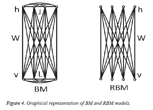
In 1985, Hinton et al. proposed a Boltzmann Machine (BM), which contains two layers named visible and hidden. The Restricted Boltzmann Machine (RBM) uses the concept of the BM. The dierence between the RBM and the BM is that the connections of the hidden and visible layers are disjointed in an RBM. That is, in an RBM there are no intra-connections between the hidden layers and the visible layers. Figure 4 illustrates the BM and RBM machines. Let v and h represent the set of visible and hidden units. The energy of the joint configuration {v, h} for BM can be defined as [22,25].

Where
• W is the weight between the visible and the hidden layers.
• L is the weight from visible to visible layer.
• J is the weight from hidden layer to hidden layer.
Since we are working on an RBM, therefore L=J=0. So we have


where

• a is the bias for the visible units
• b is the bias for the hidden units
• i is the number of visible units
• j is the number of hidden units.
The joint probability for visible and hidden units can be defined as

where Z is the partition function defined as

Through marginalising the hidden vector h we can find the probability of the vector v as

As there is no connection in the hidden unit, the binary state hj of hidden unit j is set to 1 with the probability

Given a hidden vector v, we can easily calculate the step of visible units:

Where σ (x) is the sigmoid function. Using Equations 8 and 9 and Gibbs sampling techniques, we can easily update the visible unit vectors and hidden unit vectors. The weight function can also be improved by using the following equation:

Computing < vi, hj >data is comparatively easy, whereas the computation of the value < vi, hj >model is very dicult. The value of < vi, hj >model can be calculated by sampling methods like Gibbs, Contrastive Divergence (CD), Persistent Contrastive Divergence (PCD) and Free Energy in Persistent Contrastive Divergence (FEPCD).
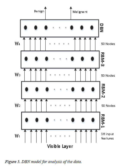
We know that a Deep Belief Network (DBN) is constructed by stacking RBM models, acting as a skeleton for the construction of the DBN. In our model, we use 4 RBM layers, RBM-1, RBM-2, RBM-3 and RBM-4. RBM-1 has 18 inputs, because we have selected 18 features. Furthermore this RBM has 50 output units. Both RBM-2 and RBM-3 have 50 input units and 50 output units. Lastly RBM-4 has 50 input units and 2 output units, as we classify our data into two classes. The whole procedure is presented in Figure 5.
The input is first fed to the visible layer, which passes its input to the first RBM named RBM-1. The data moves back and forth between the RBM-1 layer and the visible layer until RBM-1 reaches some final decision. For updating the weight values and the neuron values, the network utilises Equations 8 and 9 for calculating the final values. As RBM-1 finally calculates its values, it passes these to the next hidden layer known as RBM-2. In this case, RBM-1 works as a visible layer for RBM-2.
This same procedure is carried on throughout the network. As the network analysis proceeds, the weight value W1 is developed between the visible layer and layer RBM-1. The weight value W2 is developed between the RBM-1 layer and layer RBM-2. The weight value W3 is developed between the RBM-2 layer and RBM-3 layer, and the weight value W4 is developed between the RBM-3 layer and the DBN layer. In our model we have used back propagation for fine tuning all the parameters along with the weight values, these being W1+1, W2+2, W3+3 and W4+4. All the particulars of our model and its sampling method are summarised in Table 1.
| Parameters | RBM-1 | RBM-2 | RBM-3 | RBM-4 | Output layer |
|---|---|---|---|---|---|
| Input by output | 18 by 50 | 50 by 50 | 50 by 50 | 50 by 50 | |
| No. of epochs | 50 | 50 | 50 | 30 | 50 by 2 |
| Sampling method | CD | CD | CD | CD |
Table 1: Detailed description of each block of the machine.
Contrast-Enhancement
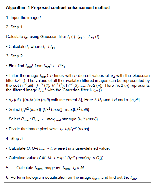
The background image information of the histopathological images coexists with the fore ground image information, and also the images suer from poor contrast. To overcome these issues we have implemented the contrast-enhancement technique of [26] with modifications such as:
• Step 1: Background subtraction
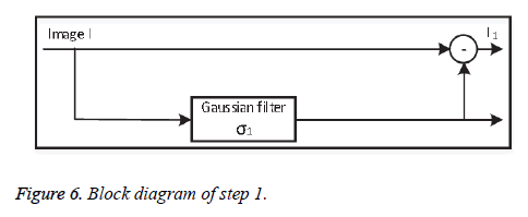
At first the original image information is subtracted from the non-uniform background information, separated using a lowpass Gaussian filter with standard deviation σ1. Depending on the value of σ1, step 1 (Figure 6) successfully removes the background variations globally.
• Step-2: Local adjustment
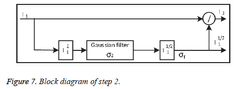
To improve the contrast information locally, the output image from step 1 is divided pixel-wise by the variance of its spatial neighbour to minimise the contrast. Dividing the whole image by the standard deviation σ2 may amplify the noise inside the images, which degrades valuable image information. Step-2 shown in Figure 7.
• Step-3: Noise control
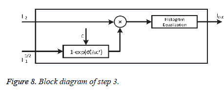
To reduce the noise amplification Khan et al. [27] proposed a correction factor M:

where p=2. Factor M multiplies the output of phase-2. Here, σf is the local standard deviation and C is a user-defined parameter which controls the background noise. Step-3 has illustrated in Figure 8.
The overall algorithm for the normalisation task (Algorithm-1) is shown below.
Feature-Extraction
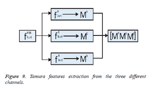
One of the important steps of image classification is extracting the features from the images. Consider fRGB (u, v)={fR (u, v), fG (u, v), fB (u, v)} be an RGB image, here R, G, B represents the Red, Green, and Blue channel information. From the image fRGB (u, v), Tamura features vector TR, TG and TB has been extracted from each of the respective channels shown as Figure 9.
Coarseness
Fineness of texture is measured by coarseness. The measure of coarseness is influenced by the scale as well as the duplication percentage of the components within that area. The largest size of the texture is also identified by coarseness [28]. To calculate the coarseness within the image, average values are calculated at all the available points by varying the window size. Centred at the point (u, v) and for a window of size 2k × 2k, the average value can be formulated as
2k × 2k non-overlapping neighbouring-window average variations have been calculated in both the horizontal and vertical directions:


Irrespective of the direction, the value of k which maximises the output values is considered an optimal value. Sbest is then calculated as

Contrast
The intensity within a texture contains a significant amount of information. Contrast represents the dierence of the level of intensity within a texture. The following four factors are considered when contrast is measured [29]:
(a) The range of Gray level within an image
(b) The polarisation of the Gray-level distribution
(c) Sharpness of edges
(d) Period of repeating patterns.
Considering the above four factors contrast can be defined as
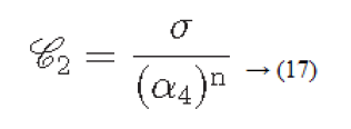
Where
α4=μ4/σ4: is known as kurtosis
μ4: Fourth moment about the mean
σ4: Variance2
Directionality
Directionality is a global property that refers to the shape of texture primitives and where they are placed within a specific region [29-31].

Hd: is the local direction histogram
no: is the number of peaks of Hd
wo: o is the range of the oth peak between valleys
o: o is the oth peak position of Hd
Line-likeness
Let PDd (i ,j) represent a directional co-occurrence matrix, where each element of this matrix is defined as “the relative frequency with which two neighbouring cells separated by a distance d along the edge direction occurs” [29,30]. Co-occurrences in the same direction are weighted by +1, and co-occurrences with directions perpendicular to each other are weighted -1. Using PDd (i, j) the line-likeness can be measured as [30].

Regularity
Regularity can be defined as

Where r is the normalising parameter [29].
Roughness
According to the results of Tamura et al.’s experiments, a combination of coarseness and contrast best aligns with the psychological results [29].

Results and Discussion
We have utilised the BreakHis dataset for our experiments, where the dataset is grouped into m={40X, 100X, 200X, 400X} groups where X represents the magnification factor. Each of the images in this dataset is RGB in nature and 700 × 460 pixels in size. We have used Tamura features as attributes and extracted the features from all the channels, which produces a total of 18 features.
The experiments have been performed on each of the individual groups of the dataset separately; 70 percent, 15 percent, and 15 percent of the data have been used for the training, validation and testing purposes, respectively. Let each group in the dataset be represented by the set Xm.
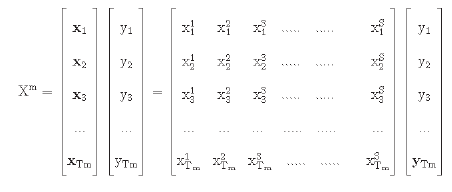
Here the value of S is equal to 18. Tm represents the total data of the group

trm=training data of group m;
tsm=test data of group m;
tvm=validation data of group m.
yi {Benign, Malignant}.
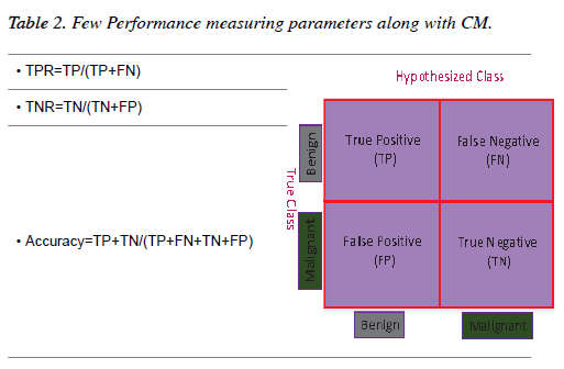
The results of all the experiments of this chapter have been evaluated through the Confusion Matrix (CM) and a few other performance-measuring parameters. A two-dimensional table which illustrates the performance of a classifier is known as a CM [32]. If a classifier provides 100% accuracy performance then all the non-diagonal elements of the CM will be zero [33]. Table 2 shows a graphical representation of a CM for a binary classifier along with a few performance-measuring parameters.
Results and comparison
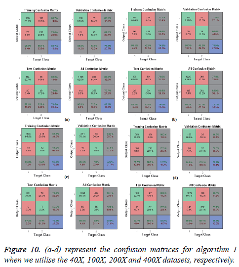
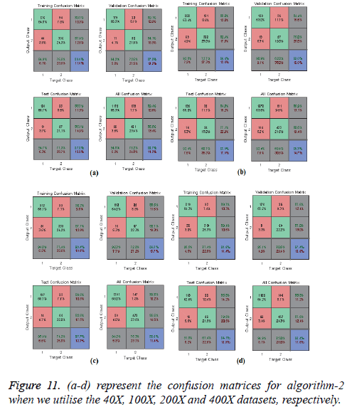
In Figures 10 and 11, the a-d images show the train, validation, test and over-all performance when we use the 40X, 100X, 200X and 400X datasets for Algorithms 1 and 2, respectively. When we use the 40X database and Algorithm 2, the train, test, validation and overall accuracies remain almost the same, at around 88.7%. When we use the 100X dataset, the Test shows less accuracy than the train and validation performance. When we use the 200X dataset, the train, validation, test and overall accuracies are 89.4%, 86.3%, 87.7% and 86.8%, respectively. When we use the 400X database, the overall accuracy achieved is around 88.4%. These confusion matrices also show that, when we utilised Algorithm 1 for the 40X, 100X, 200X and 400X magnification-factor database, 15.5%, 22.60%, 29.90% and 14.6% of the malignant images have been misclassified as benign images. However, 24.30%, 36.10%, 50.50% and 26.9% of the benign images have been wrongly classified as malignant images. The overall accuracy achieved for the 40X, 100X, 200X and 400X cases was 82.20%, 74.70%, 69.00% and 81.70%, respectively; for all magnification factors a greater percentage of the database has been misclassified as benign. When we utilised Algorithm 2, 10.60%, 13.10%, 10.02% and 11.20% of the malignant data were misclassified as benign images for the 40X, 100X, 200X and 400X cases, respectively. On the other hand, 13.40%, 19.40%, 14.50% and 12.40% of the data has been classified as malignant though they are originally benign images for the 40X, 100X, 200X and 400X cases, respectively.
Performance: The Mean-Square Error (MSE) assesses the quality of a model and a good classifier is expected to have a small MSE. Let θ be the predicted value, θ be the observed value for n observations, then the MSE error can be defined as

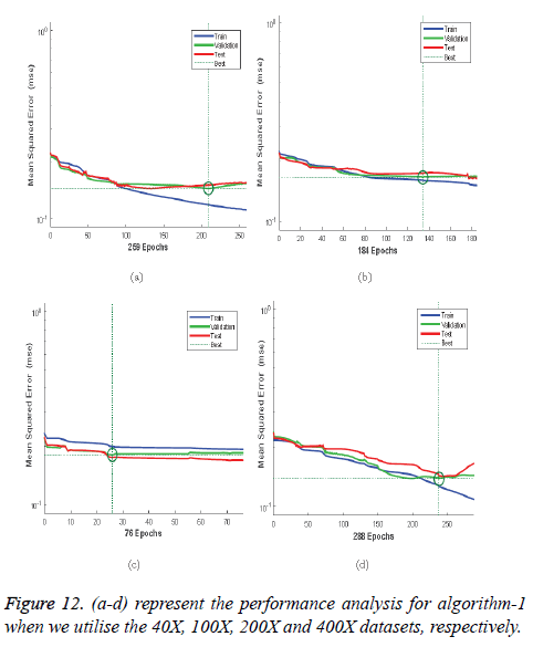
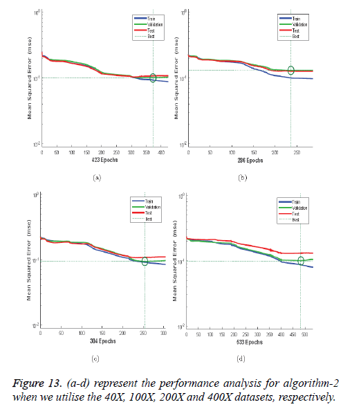
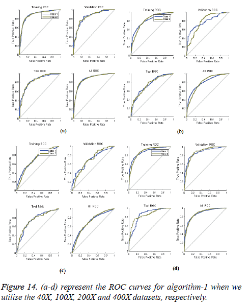
Figures 12a-12d illustrates the performance of the 40X, 100X, 200X and 400X datasets when we use Algorithm 1. Figures 13a-13d depicts the performance of the 40X, 100X, 200X and 400X datasets when we use Algorithm 2. Table 3 summarises the MSE values and the required number of epochs to achieve that value.
| Algorithm | Magnification factor | MSE | Epoch |
|---|---|---|---|
| Algorithm-1 | 40X | 0.14481 | 209 |
| 100X | 0.16528 | 134 | |
| 200X | 0.18074 | 26 | |
| 400X | 0.13813 | 238 | |
| 40X | 0.09941 | 373 | |
| Algorithm-2 | 100X | 0.09384 | 236 |
| 200X | 0.09384 | 254 | |
| 400X | 0.09948 | 483 |
Table 3: MSE values and the corresponding epoch values.
Table 3 and Figures 12 and 13 shows that, for Algorithm 1, the best MSE values are achieved when we use the 400X magnification factor, and it takes 209 epochs. However, when we have recourse to Algorithm 1 and the 200X magnification factor dataset the model requires 26 epochs to achieve an MSE of 0.18074. Though it requires fewer epochs, it performs worse than all the other datasets when we exploit Algorithm 1. When we utilise Algorithm 2 almost all the datasets show the same kind of MSE, which lies in between 0.09384 and 0.09948. However, when we implement the 400X database it requires 483 epochs, which is larger than for the other three datasets.
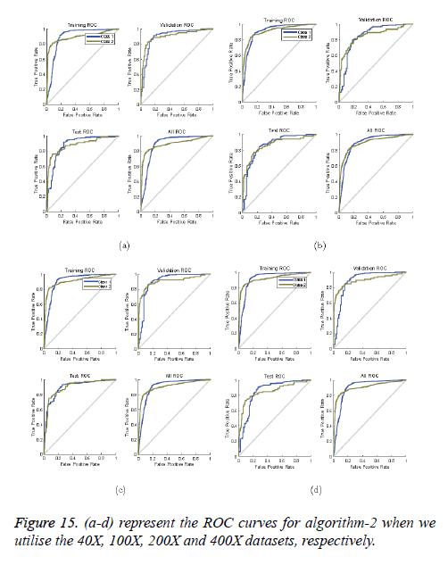
ROC curves: ROC curves show the false positive rate and true positive rate performance. The best performance is achieved at the top-most left position. That position indicates that the false positive rate is 0 and the true positive rate is 1, which also indicates that the true negative rate is 100.00%. Figures 14 and 15 show ROC curves for the Algorithms 1 and 2, respectively.
So far, very little work has been done on classifying the BreakHis dataset. Fabio et al. used the Local Binary Pattern (LBP), Local Plane Quantization (LPQ), Gray-Level-Co-occurrence Matrix (GLCM), Parameter Free Threshold Adjacency Statistics (PFTAS) method for feature-extraction. These authors applied four dierent classifiers: 1-Nearest Neighbor (1- NN), Quadratic Linear Analysis (QDA), Support Vector Machine (SVM) and Random Forest (RF). Overall they achieved the best performance when they used the PFTAS descriptor and SVM classifier, and their achieved performance Accuracy was 85.1 ± 3.1%. As a descriptor, we use Tamura features. Our proposed Algorithms 1 and 2 both use the RBM method for image classification. When we use Algorithm 1, the overall accuracy achieved is 82.20%, 74.70%, 69.00% and 81.70% for the 40X, 100X, 200X and 400X datasets, respectively, while Algorithm 2 gave 88.70%, 85.30%, 88.60% and 88.40% accuracy for the 40X, 100X, 200X and 400X databases, respectively (Table 4).
| Descriptor | Classifier | Magnification factor and accuracy % | |||
|---|---|---|---|---|---|
| 40X | 100X | 200X | 400X | ||
| CLBP [34] | SVM | 77.4 ± 3.8 | 76.4 ± 4.5 | 70.2 ± 3.6 | 72.8 ± 4.9 |
| GLCM [34] | RF | 73.6 ± 1.5 | 76.0 ± 1.9 | 82.4 ± 2.3 | 79.8 ± 2.5 |
| LBP [34] | SVM | 74.2 ± 5.0 | 73.2 ± 3.5 | 71.3 ± 4.0 | 73.1 ± 5.7 |
| LPQ [34] | 1-NN | 72.8 ± 4.9 | 71.1 ± 6.4 | 74.3 ± 6.3 | 71.4 ± 5.2 |
| ORB [34] | QDA | 74.4 ± 1.7 | 66.5 ± 3.2 | 63.5 ± 2.7 | 63.5 ± 2.2 |
| PFTAS [34] | SVM | 81.6 ± 3.0 | 79.9 ± 5.4 | 85.1 ± 3.1 | 82.3 ± 3.8 |
| Algorithm 1 | RBM | 82.2 | 74.7 | 69.0 | 81.7 |
| Algorithm 2 | RBM | 88.7 | 85.3 | 88.6 | 88.4 |
Table 4: Comparison of results using our proposed algorithm and other algorithms.
In [34] the performance has been evaluated through the accuracy measure. However, in this chapter we have found the ROC information and the error performances with the epoch.
Conclusion
In this chapter we have proposed an automatic BC image classifier framework which has been constructed using stateof- the art deep neural network techniques. Instead of using raw images we have utilised Tamura features, as they provide textural information. As a deep-learning tool we have implemented an unsupervised restricted Boltzmann machine which contains four layers and is guided by a supervised backpropagation technique. For the back-propagation, scaled conjugate gradient techniques have been utilised. We have performed our experiments on the BreakHis dataset and obtained 88.7%, 85.3%, 88.6% and 88.4% accuracy for the dataset of 40X, 100X, 200X and 400X magnification factors, respectively. Most of the experiments on the BreakHis dataset judged the performance on the basis of accuracy; however, in this chapter we have also considered TPR, FPR values along with a detailed description of the ROC curves. The error performance as a function of the epoch is also explained in detail. This chapter shows that the RBN method is very eective for automatic breast-cancer image diagnosis. However, in the future the combination of CNN and RBM will enhance the classification performance.
References
- Rajesh K, Rajeev S, Srivastava S. Detection and classification of cancer from microscopic biopsy images using clinically significant and biologically interpretable features. J Med Eng 2015; 2015: 1-14.
- Diz J, Marreiros G, Freitas A. Using data mining techniques to support breast cancer diagnosis. N Contrib Info Sys Technol 2015; 689-700.
- Zhang Y, Zhang B, Lu W. Breast cancer classification from histological images with multiple features and random subspace classifier ensemble. AIP Conference Proc 2011; 1371: 19-28.
- Bruno DOT, do Nascimento MZ, Ramos RP, Batista VR, Neves LA, Martins AS. LBP operators on curvelet coefficients as an algorithm to describe texture in breast cancer tissues. Exp Sys Appl 2016; 55: 329-340.
- Paul A, Dey A, Mukherjee DP, Sivaswamy J, Tourani V. Regenerative random forest with automatic feature selection to detect mitosis in histopathological breast cancer images. Cham Springer Int Publ 2015; 94-102.
- de Oliveira Martins L, da Silva EC, Silva AC, de Paiva AC, Gattass M. Classification of breast masses in mammogram images using ripleys k function and support vector machine. Berlin Heidelberg Springer Berlin Heidelberg 2007; 784-794.
- Chang RF, Wu WJ, Moon WK, Chou YH, Chen DR. Support vector machines for diagnosis of breast tumors on US images. Acad Radiol 2003; 10: 189-197.
- Kavitha S, Thyagharajan KK. Features based mammogram image classification using weighted feature support vector machine. Berlin, Heidelberg: Springer 2012; 320-329.
- Chang RF, Wu WJ, Moon WK, Chen DR. Improvement in breast tumor discrimination by support vector machines and speckle-emphasis texture analysis. Ultrasound Med Biol 2003; 29: 679-686
- Zhang YD, Wang SH, Liu G, Yang J. Computer-aided diagnosis of abnormal breasts in mammogram images by weighted-type fractional fourier transform. Adv Mech Eng 2016; 8; 1687814016634243.
- Dheeba J, Selvi ST. Classification of malignant and benign microcalcification using SVM classifier. 2011 International Conference on Emerging Trends in Electrical and Computer Technology 2011; 686-690.
- El-Naqa I, Yang Y, Wernick M, Galatsanos N, Nishikawa R. A support vector machine approach for detection of microcalcifications. IEEE Trans Med Imag 2002; 21: 1552-1563.
- Dawson A, Austin R, Weinberg D. Nuclear grading of breast carcinoma by image analysis: classification by multivariate and neural network analysis. Am J Clin Pathol 1991; 95: 29-37.
- Krizhevsky A, Sutskever I, Hinton GE. Image net classification with deep convolutional neural networks. Adv Neural Info Proce Sys 2012.
- Su H, Liu F, Xie Y, Xing F, Meyyappan S, Yang L. Region segmentation in histopathological breast cancer images using deep convolutional neural network. IEEE 12th International Symposium on Biomedical Imaging (ISBI) 2015; 55-58.
- Wu CY, Lo SCB, Freedman MT, Hasegawa A, Zuurbier RA, Mun SK. Classification of microcalcifications in radiographs of pathological specimen for the diagnosis of breast cancer. Acad Radiol 1995; 2: 199-204.
- Fonseca P, Mendoza J, Wainer J, Ferrer J, Pinto J, Guerrero J, Castaneda B. Automatic breast density classification using a convolutional neural network architecture search procedure. Conference: Conference: SPIE Medical Imaging Orlando USA 2015.
- Spanhol FA, Oliveira LS, Petitjean C, Heutte L. Breast cancer histopathological image classification using convolutional neural networks. International Joint Conference on Neural Networks (IJCNN) 2016; 2560-2567.
- Xu J, Luo X, Wang G, Gilmore H, Madabhushi A. A deep convolutional neural network for segmenting and classifying epithelial and stromal regions in histopathological images. Neurocomputing 2016; 191: 214-223.
- Sirinukunwattana K, Raza S, Tsang YW, Snead D, Cree I, Rajpoot N. Locality sensitive deep learning for detection and classification of nuclei in routine colon cancer histology images. IEEE Trans Med Imag 2016; 35: 1196-1206.
- Kooi T, Litjens G, van Ginneken B, Gubern-Mrida A, Snchez CI, Mann R, den Heeten A, Karssemeijer N. Large scale deep learning for computer aided detection of mammographic lesions. Med Image Anal 2017; 35: 303-312.
- Hinton GE, Osindero S, Teh YW. A fast learning algorithm for deep belief nets. Neural Comput 2006; 18: 1527-1554.
- Liu Y, Zhou S, Chen Q. Discriminative deep belief networks for visual data classification. Patt Recogn 2011; 44: 2287-2296.
- Abdel-Zaher AM, Eldeib AM. Breast cancer classification using deep belief networks. Expert Syst Appl 2016; 46; 139-144.
- Gao J, Guo Y, Yin M. Restricted Boltzmann machine approach to couple dictionary training for image super-resolution. 2013 IEEE International Conference on Image Processing 2013; 499-503.
- Khan MAU, Soomro TA, Khan TM, Bailey DG, Gao J, Mir N. Automatic retinal vessel extraction algorithm based on contrast-sensitive schemes. International Conference on Image and Vision Computing New Zealand (IVCNZ) 2016; 1-5.
- Khan TM, Bailey DG, Khan MAU, Kong Y. Ecient hardware implementation strategy for local normalization of fingerprint images. J Real Time Image Proc 2016; 1-13.
- Howarth P, Ruger S. Evaluation of texture features for content-based image retrieval. Berlin, Heidelberg: Springer Berlin Heidelberg 2004; 326-334.
- Tamura H, Mori S, Yamawaki T. Textural features corresponding to visual perception. IEEE Trans Sys Man Cybern 1978; 8: 460-473.
- Bianconi F, lvarez Larrn A, Fernndez A, Discrimination between tumour epithelium and stroma via perception-based features. Neurocomputing 2015; 154: 119-126.
- Wang Z, Liu H, Qian Y, Xu T. Crowd density estimation based on local binary pattern co-occurrence matrix. 2012 IEEE International Conference on Multimedia and Expo Workshops 2012; 372-377.
- Marom ND, Rokach L, Shmilovici A. Using the confusion matrix for improving ensemble classifiers. Electric Electron Eng Israel (IEEEI) 2010; 000555-000559.
- Wu SH, Lin KP, Chien HH, Chen CM, Chen MS. On generalizable low false-positive learning using asymmetric support vector machines. IEEE Trans Knowl Data Eng 2013; 25: 1083-1096.
- Spanhol FA, Oliveira LS, Petitjean C, Heutte L. A dataset for breast cancer histopathological image classification. IEEE Trans Biomed Eng 2016; 63: 1455-1462.
