- Biomedical Research (2016) Volume 27, Issue 3
Deformable registration of 4D-CT lung image using landmark tracking.
JunhaWu1, Bingfeng Hu1, Xuan Yang2*
1National High Performance Computing Center at Shenzhen, Shenzhen University, Shenzhen, Guangdong, China
2College of Computer Science and Software Engineering, Shenzhen University, Shenzhen, Guangdong, China
- *Corresponding Author:
- Xuan Yang
College of Computer Science and Software Engineering
Shenzhen University
China
Accepted date: February 29, 2016
Abstract
Landmark based image registration algorithms have been applied to medical image analysis widely. While estimation of the correspondence between landmarks among images are the most important and difficult problem. In this paper, novel landmarks based image registration method combining local tracking and global adjustment of landmarks in 4D-CT lung images is proposed. In order to accurately establish the corresponding landmarks in images at different phases of 4D-CT, we introduce spatial information to structure tensor and use structure tensor to track landmarks in images at different phases. The prior knowledge of respiratory motion is utilized to limit the search area of corresponding landmarks. Further, a cost function measuring similarity of images, bending energy of transformations and spatio-temporal smoothness of trajectories of landmarks along respiratory phases is given. We update the tracked results of landmarks by minimizing a cost function. After the optimization, the correspondence between landmarks is improved and the trajectories of landmarks are enforced to be more smooth, thus, more accurate registration results can be achieved. Experimental results of public lung dataset demonstrate the effectiveness of the proposed method.
Keywords
Image registration, Structure tensor, Object tracking, Landmark correspondence.
Introduction
Four Dimensional Computed Tomography (4D-CT), developed for radiotherapy treatment planning, is an imaging technique that allows for the acquisition of time varying 3D image sequences of the thorax through the respiratory cycle [1,2]. 4DCT lung image can be used to estimate respiratory motion model, and then guides radiation therapy in clinical treatment [3,4]. It is a challenge for estimating lung motion model using 4D-CT images, since 4D-CT images contain artefacts such as noisy and lower spatial resolution. Moreover, 4D-CT image contains respiratory induced CT characteristics of the pulmonary parenchyma that will reflect the changes in air content [3]. The respiratory motion is non-uniform from lung expansion to lung contraction, hence, deformable image registration is an effective technique to estimate motion model of lung.
For deformable image registration, there are two main categories. One is intensity based, which aims at aligning dense image intensities of images [4-8]. Intensity based algorithms works better when the register images are very similar (small deformation), but lead to mis-registration for large deformation in images. The other one is landmark based, which attempts to find the correspondence of landmarks between images [9-12], those landmarks mainly including surfaces [13], lines [14] and points [9,15]. Especially, commonly used point landmarks are the unique points in intensity map, such as tip like, saddle like and sphere line structure. Compared to intensity based image registration algorithms, landmark based image registration algorithms avoid solving large system of equations and can handle image registration problem with large deformation. Moreover, landmark based methods are also more flexible because registration features can be customized for the particular study [16]. In order to establish correspondence of landmarks among images, there are manually identifying method [15] and automatically identifying method [17,18]. While manually identifying method is time consuming and introduces errors, which leads to difficult to find true consistent landmarks.
Many researchers proposed methods to automatically establish landmarks correspondence between on one image to another. The automatic landmarks identification algorithms can be divided into two categories: local algorithms and global algorithms. Local algorithms are to establish correspondence of each landmark independently, instead of establishing the correspondence of one landmark based on the correspondence of other landmarks. Tracking and trajectory fitting for landmarks are commonly used methods to find the corresponding positions of landmarks in an image sequence. Most tracking methods are classical template based [19]. Fan et al. [20] employed mean shift algorithm to track landmarks in a 3D image sequence. Xiong et al. [21] detected natural junction structures in the lung and described trajectories of these landmarks by closed B-splines to estimate the lung motion. Castillo et al. [22] included general polynomials into the optical flow equation to calculate a parameterized trajectory of a point by utilizing all available spatial and temporal image information from a local window located at the point.
Global algorithms apply deformable registration to track landmarks positions. Frangi et al. [23] provided a generic framework for automatic selection of corresponding landmarks in 3D shapes, and propagate landmarks in one respiratory phase to the others. Paquin et al. [18] proposed a hybrid multiscale landmark and deformable registration algorithm to make image matching robust with respect to the location of landmarks. Compared with local algorithms, global algorithms establish the correspondence of all landmarks at the same time. Correspondence of each landmark is influenced each other. Global algorithms can acquire more accurate global alignment of landmarks and prevent severe mismatch of isolated landmarks. However, it should be mentioned that global algorithms may compromise the alignment of local structures, because it needs to find a medium between local align accuracy and global align accuracy.
In this paper, we propose a novel local global tracking method applied to track landmarks at different phases of 4D-CT images, which combines both the alignment of local structures and alignment of global images. First, landmarks are given in the image at the reference phase, structure tensor based approach is employed to track these given landmarks independently in images at all phases. Since structure tensor has advantages of powerful local patch descriptor, low dimension, multi-scale and anti-noise over other tracking methods, it is capable of tracking landmarks in 4D-CT lung images with complex structures and noise. However, structure tensor describes a local patch by summing all structure tensor matrices inside a local region, which results in an isotropy descriptor. That is, structure tensor cannot be used to identify local structures that are similar to each other in structure but are different in orientation. To tackle this issue, spatial information is introduced to structure tensor in this paper. Besides, we make use of the prior knowledge of respiratory motion to limit the searching area during tracking. The accuracy of landmark tracking has been improved significantly by the improved tracking algorithm based on structure tensor. Although the accuracy of tracking of individual landmark has been improved, there are still isolated landmarks that are mismatched. This is the problem existed in local algorithms inherently because each landmark is tracked independently rather than being constrained by each other. So a spatiotemporal constraint optimization model, which mainly contains the similarity between local regions of images and the spatiotemporal smoothness of deformation function, is proposed in this paper also. An optimization procedure is performed to update the tracking results of landmarks, and the corresponding accuracy of landmarks is improved as a whole and the trajectories of landmarks are constrained to be smooth in temporal dimension.
Landmark Tracking Based on Structure Tensor
The 4D-CT image acquired with N phases is denoted as I={It| t=0,1,….,N-1}. Supposing that I0 is the reference image, and there are k landmarks in I0. For each landmark poj, j=1,….,k, our goal is to track corresponding positions corresponding positions ptj in target images {It|t=1,2,…,N-1}. For 4D-CT lung images, anatomy based landmarks, such as junction structures, bifurcation points and corners are often preferred, because the statistics of intensity values and geometrical structures over the neighbourhood region of these landmarks will not significantly change during the respiration cycle. The small neighbourhood region centered at a landmark can be taken as a template, and then the corresponding region in a successive image It, t=1, …,N-1 is found in the sequence according to a similarity measure.
Structure tensor
Structure tensor is served as a powerful analysis tool that can effectively model and estimate the low level feature dependencies, orientation and position of feature pattern. Donoser et al. [24] expanded structure tensor as local patch descriptor to track interested objects in video. We also employed structure tensor to describe characteristics of the local patch centered a landmark, and use this descriptor to track the small neighbourhood region with similar characteristics in an image sequence. The centers of the searched regions are the corresponding landmarks in different phases. The structure tensor of a point x in the image I is defined as follows,
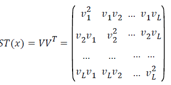 (1)
(1)
Where V=[ν1,….,νL] is the L dimensional features vector of x with low level features, such as intensity and derivatives, to be considered. Since second order derivatives of vessels have more physical meanings, we define a specified seven dimensional features vector as,
 (2)
(2)
where I is the intensity of x, and the others are the second partial derivatives in different directions at x. The seven dimensional features vector can be used to generate structure tensor that describes the vessels structures in a local region. For a local patch Px centered at x in the image I, every point in Px can be describe by a structure tensor matrix, correspondingly, the local patch can be described by summing all the structure tensor matrices of all points in Px as descriptor SP(x),
 (3)
(3)
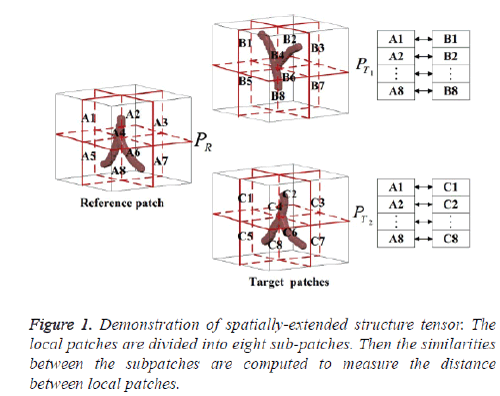
The structure tensor of a local patch is a feature descriptor which can be used to find the local patch with similar features. However, it cannot be used directly in landmark tracking for 4D-CT lung images. The reason is that the structure tensor of a local patch contains average information of the local patch, which is not sensible to the local structures that are similar in shape but are different in orientation. In a 4D-CT lung image, there are many similar vessels intersections structures, which make it difficult to distinguish one from another. As illustrated in figure 1, three synthetic vessel structures in 3D are shown. The left one PR is the template patch and the right PT1 and PT2 are two local patches similar to the left one in shape. Based on the structure tensor, all these three patches are similar to each other. Indeed, in 4D-CT images, PT1 is different from PT2. Then, it can be guessed that landmarks tracking based on traditional structure tensor may lead to biased results for 4D-CT lung images.
Spatially-extended structure tensor
We introduce spatial information into the traditional Structure Tensor (ST) to tackle the isotropic issue, named Spatially Extended Structure Tensor (SEST). We combine the structure tensor with spatial information to enhance the identification ability of structure tensor. Given a 3D local patch Px centered at x, we uniformly partition the local patch into 8 subpatches Px,i, i=1,…,8. Let SPi be the structure tensor of the ith sub patch Px,i, then, the SESP(x) is defined as,
SESP(x)=[SP1 SP2 … SP8]7 × 56 (4)
Where SPi, i=1,…,8 is a 7 × 7 structure tensor matrix.
The spatially extended structure tensor can distinguish the two patches shown in figure 1. As shown in figure 1, the reference patch PR is uniformly divided into 8 local sub patches A1, A2, …, A8. Similarly, the right two patches PT1 and PT2 are partitioned as B1, B2, …, B8 and C1, C2, …, C8 in the same way.
It can be observed that Ai is similar to Ci and is different from Bi,i=1, …, 8. Correspondingly, the patch PR is similar to PT2 instead of PT1 based on the similarity of subpatches. That implies that SEST can be used to distinguish local structure similar in shape but different in orientation.
Landmark tracking using spatially extended structure tensor
To measure the similarity between local patches, it is required to define a valid distance measure between structure tensor matrices. Forserter et al. [25] formulated metric to measure distance between matrices in connected Riemannian manifold. But before measuring matrices distance, we should calculate a time consuming similarity scores. Donoser et al. [24] adapt a method proposed by Kluckner et al. [26] to approximate the matrices for more efficient calculation. The approximated representation relies on repeated random sampling theory and Monte Carlo simulations. Structure tensor is a symmetric positive semi definite matrix, the Cholesky decomposition ST=UUT can be used to decompose structure tensor to obtain a lower triangular matrix U. The low triangular matrix maps the standard basis vector b ϵ B, B={ei:1 ≤ i ≤ N}of a L-dimensional Euclidean space to a vector a, a=U b, a ϵ RL. The vector represents the characteristics of the structure tensor ST. The Euclidean distance between vectors is the similarity measure between different structure tensor. Similar idea can be used to approximate the spatially extended structure tensor. Given a spatially extended structure tensor, SESP(x)=[SP1 SP2 … SP8], SPi can be decomposed as SPi=UiUT i, i=1,…,8. Each Ui is represented as a vector ai ϵ RL, all ai are cascaded as a long vector sa=[aT1, aT2, …, aT8]T to represent the spatially extended structure tensor. The Euclidean distance between vectors sa is the similarity measure between different spatially extended structure tensors.
The tracking procedure of each landmark p0j, j=1, …, k, using SEST is illustrated as Algorithm 1. During this procedure, the searching area of SEST is different from that of ST.
Algorithm 1: tracking algorithm based on spatially extended structure tensor
Set local patch size l × w × h and the search area size sl × sw × sh;
Compute SEST (p0j) of the local patch centered at p0j;
for t=1:N-1 do
Let p0j be the initial position of ptj;
for each ptj in the search area do
Compute SEST(ptj) of the local patch centered at ptj in image It;
Compute D(ptj)=||SEST(p0j)-SEST(ptj)||;.
Update ptj in the search area linebyline;
end for
Find the position minimizing D(ptj) as the tracked position of p0j in It
end for
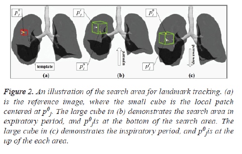
is different from that of ST. We know ST is generally used to track objects in video, where the movement and the trajectory of the interested object is uncertain and unexpected. Then, it is needed to search the candidate object along different directions alternatively using ST. However, during respiratory motion, the vessels intersections move slightly and regularly compared to objects in video. So the search area can be limited in a small region. In expiratory period, lung expands downward; in inspiratory period, lung contracts upward. Hence, compared with ST tracking algorithm, there is no need to search the object in both up and down directions for SEST tracking algorithm. As shown in figure 2, the local patch centered at p0j in figure 2a is the template, and the cubes in figures 2b and 2c are the searching areas of the template at two different phases. What we should do is to search the template upward during expiratory period (Figure 2b), where p0j is at the bottom of the search area, and downward during inspiratory period figure 2c, where p0j is at the up of the search area. The limited search area reduces the possibility of mistracking and saves tracking time.
Figure 2: An illustration of the search area for landmark tracking. (a) is the reference image, where the small cube is the local patch centered at p0j. The large cube in (b) demonstrates the search area in expiratory period, and p0j is at the bottom of the search area. The large cube in (c) demonstrates the inspiratory period, and p0j is at the up of the each area.
Optimization of Tracking Results
Cost function
After tracking landmarks individually, it is inevitable that there exist tracking errors for several landmarks due to the noise and artefacts in 4D-CT images. That is, there might be the tracked positions of several landmarks obviously deviating from their correct positions. So, it is needed to update the tracking results of landmarks in images at different phases in a global sense. An optimization procedure is performed to update the tracking results of landmarks according to the similarity between images and the spatiotemporal smoothness of global deformation function. To update tracking results of landmarks in a global sense, it is needed to deform the 3D images I0 by the transformation function ft based on the correspondence between {p0j} and {ptj}, t=1, …, N-1. We employ the Thin Plate Splines (TPS) [27] to be the transformation by considering {p0j}as the source landmarks in the I0 and {ptj} as the target landmarks in It have the property that each landmark has a global influence on the transformation. That is, if the position of one landmark is updated, then all other voxels in the image are adjusted as well. This can be an advantage to update the tracking results of landmarks in a global sense.
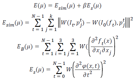
Optimization of tracking results are based on following criteria: 1) the deformed image should be aligned to the target image as a whole, rather than that only the landmarks are corresponding to each other; 2) the spatial bending energy of the spatial transformation should be less; 3) the trajectories of voxel in the 3D image should be smooth also. To update the tracking results of landmarks satisfying the constraints described above, a spatiotemporal cost function is proposed as follows,
 (5)
(5)
Where μ={p1j} U…U {pjN-1}, j=1,2,…,k are all tracked results of landmarks {p0j} in images at different phases. W is a neighborhood window of wl × ww × wh voxels. x=(x1, x2, x3) is the position of a voxel in a 3D image. φ(x, t) is the trajectory of the voxel x along temporal dimension by sequentially connecting the deformed position ft(x), t=1,…,N-1 along respiratory phases. α and β balance the second and the third terms. To get better α and β, we do a lot of experiments. Finally, we set α and β to be le-3.
The value of the cost function is determined by the transformations {ft, t=1,…,N-1}, which are influenced by landmarks μ. The goal of optimization is to adjust all tracked results of landmarks μ to let the value of the cost function E approach to global minima as much as possible. There are three energy terms in the spatiotemporal cost function. The first term Esim measures the similarity between the target image It and the image I0(ft) deformed by the transformations ft. Specifically, the similarity is evaluated in each landmark’s neighbourhood W instead of the whole image, by integrating all differences between the intensity of every neighbouring voxel in W(It, ptj) and the intensity of the corresponding voxel in W(I0(ft), ptj). The second energy term EB is a bending energy constraint for the transformation ft. We use Laplacian operator to impose spatial smoothness. Similar to the first term, the bending energy is evaluated in each landmark’s neighbourhood W, by integrating all bending energy of every neighbouring voxel in W(ft). The third energy term ES is a temporal smoothness constraint for the trajectories of voxels in the neighbourhood of a landmark. It is known that the deformation of pulmonary organ from one time point to another time point is subtle in space, and the motion trajectory of every voxel should be a smooth curve. Similar to the second term, the temporal smoothness of a trajectory is evaluated by the Laplacian operator along temporal dimension.
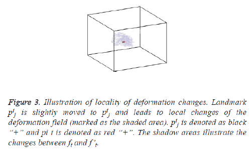
It is noted that the three parts in the cost function is defined on the transformations ft, and evaluated in each landmark’s neighbourhood cube. Although the transformations ft, have the property that each landmark has a global influence on the transformation when spacing between landmarks is small, changes of the deformation field is limited to a local neighbourhood region instead of occurring in the whole image area when only one landmark is updated. The changes of the deformation field occur in the local region surrounding the updated landmark mostly. An example is shown in figure 3, suppose the current landmark are μ={p1j} U…U {pjN-1}, j=1,2, …,k. Correspondingly, the transformations between the reference image and the image at other phases are {f1,…,ft-1,ft+1,…,}. Then, the jth landmark ptj at t phase is updated to ptj. The transformations {f1,…,fk} are updated as {f1,…,ft-1,ft+1, …,} also, where only the tth transformation function is updated. We subtract ft from f”t and show the subtraction results in figure 3. It can be seen that the changes of the deformation field after updating ptj are limited in a local region surrounding ptj instead of occurring in the whole image. This result is exactly in agreement with the local region cube used in the cost function. So, it is reasonable to evaluate the changes locally, as well as the terms used in the cost function.
Optimization
The goal of optimization is to adjust arguments to let the value of cost function approach to global minima as much as possible. Optimization can be defined as follows
 (6)
(6)
where variables μ are all coordinates of current updated landmarks. Each coordinate of each landmark corresponds to a variable. 3k(N-1) is the total number of variables in μ. Optimization of E(μ) is handled by a quasi-Newton approach in the form of the Limited memory BFGS (LBFGS) method [28]. LBFGS is an optimization algorithm for unconstrained optimization, which approximates the Broyden Fletcher Goldfarb Shanno (BFGS) algorithm using a limited amount of memory. BFGS is a kind of quasi-Newton methods with high precision and improved convergence rate compared to simple gradient descent algorithms. In BFGS, a dense 3(L-1)k × 3(L-1)k matrix is adopted to approximate inverse Hessian matrix. Since the number of variables in μ is large, it is unwisely to imply BFGS to perform optimization. Unlike the original BFGS, LBFGS represents the approximation implicitly by maintaining a history of the past m updates of μ and gradient ∇E, where generally the history size m can be less than 10. These updates are used to implicitly do operations requiring the inverse Hessian product. The LBFGS optimization requires the gradient of the cost function with respect to μ, which is approximated by the finite difference. We denote the gradient of the cost function as ∇E= (a1, . . . , a3kN ). The ∇E is calculated by,
 (7)
(7)
Where ei denotes the ith unit vector, μi is the ith variable. μi +hei represents that the ith coordinate is shifted slightly, and other coordinates are kept fixed. That means only one landmark is updated slightly and all other landmarks are fixed. Next, the new transformation fʹt is estimated based on the updated landmarks, and the new cost function value E(μi+hei) is also calculated. It must be pointed out that when only one landmark is shifted, the deformation field will change locally upon fixing other landmarks (the fixed landmarks are required to overlay the image uniformly and densely). That is, the cost function evaluates the transformation locally, which reflects the locality of the deformed results when gradient of the cost function is calculated.
Results and Analysis
Ten individual patients’ lung CT images provided by DIR-lab dataset are used to evaluate our method. Each case includes the set of 10 phases CT 16-bit integer images from T00 to T90. Images from T00 to T50 are successively acquired in inspiratory period and others from T60 to T90 are successively acquired in expiratory period. For each case, 75 corresponding landmarks from T00 to T50 are provided by experts, and also 300 corresponding landmarks in the maximum inhalation and the maximum exhalation are provided by experts. We first segment lung parenchyma from 4D-CT lung images and map 16-bit data to 8bit data to enhance the intensity of parenchyma. To make it easier to align vessel intersections during the registration, the vessels in parenchyma is enhanced by multiscale hessian filters [29]. However, the vesselness response of Hessian filter is not continue, even more is fragmentary. We use the nonlinear diffusion equation proposed by Perona and Malik [30] to make the enhanced vascular structures continuous and smooth.
Tracking results
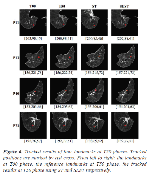
To demonstrate the tracking performance of our method, landmarks marked by experts at T00 phase are tracked from T10 to T50 respectively for the first five cases. In the image at T00 phase, a local patch centered at a landmark with size of 11 × 11 × 7 is selected as a tracking template. The search area size is 21 × 21 × 21 for the ST algorithm and is limited to 21 × 21 × 11 for the SEST algorithm. In the optimization process, a window W in size of 25 × 25 × 25 is used in the cost function. Figure 4 demonstrates the tracked results for four landmarks at T50 phase. The first column shows four landmark locations at T00 phase, and the second column shows the manually identified landmarks at T50 phase. The third and fourth columns present the tracked results at T50 phase using the ST algorithm and the SEST algorithm respectively. We expect that the tracked position is closer to the manually identified position as close as possible. The coordinate below each slice is the coordinate of the point marked by red plus. P11, P13, P40 and P73 are indices of the four landmarks. From the coordinates of points, we can see the displacement of these four landmarks is obvious. Moreover, there are similar landmarks near these landmarks, which make it difficult to be tracked. Noted that the tracked results using the SEST algorithm is more accurate than that using the ST algorithm. Especially, in the case shown in the last line, the landmark needed to be tracked is located on a vessel bifurcation, and there is a similar bifurcation near the bifurcation. The tracking result by the ST algorithm is misled by the similar structure, while the tracking result by SEST algorithm is correct exactly. This example demonstrates the performance of the SEST algorithm for tracking object in complex background.
To quantitatively evaluate the tracking accuracy of our method, tracking error is evaluated by computation of the Euclidean distance between the landmark positions marked by experts and tracked results. The tracking errors of 75 landmarks for the first five cases of DIR-lab dataset are listed in table 1. From this table, it can be obviously seen that the performance of the SEST algorithm is better than the ST algorithm in tracking error significantly. Especially, the respiratory motions in case 3, 4 and 5 are more violent than the other two cases. The improvement of tracking errors using the SEST algorithm for these three cases is significant. Moreover, standard deviation of tracking errors using the ST algorithm is larger than that using the SEST algorithm, which implies that the tracked results of some landmarks using the ST algorithm deviate from the correct positions severely. It also implies that SEST algorithm is more advantageous than ST algorithm.
| Case-1 | Case-2 | Case-3 | Case-4 | Case-5 | |
|---|---|---|---|---|---|
| Initial | 2.18(2.54) | 3.78(3.69) | 5.05(3.81) | 6.69(4.72) | 5.22(4.61) |
| ST | 0.97(1.16) | 0.91(1.07) | 1.21(1.32) | 1.80(2.03) | 2.32(2.45) |
| SEST | 0.86(1.13) | 0.76(0.97) | 0.91(1.10) | 1.28(1.29) | 1.29(1.71) |
| Improvement | 0.11(0.03) | 0.15(0.10) | 0.30(0.22) | 0.72(0.74) | 1.03(0.73) |
Table 1: Mean and standard deviation of tracking errors in mm for 75 landmarks from T00 to T50.
Optimization Results
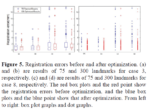
Tables 2 and 3 list the tracking errors of 75 landmarks and 300 landmarks before and after optimization respectively to compare the performance of our method with optimization and without optimization. It is observed that the tracking errors decrease slightly whether for 75 landmarks or 300 landmarks. Moreover, the standard deviation of tracking errors decrease also. Especially, the mean and standard deviation of tracking errors for case 8 is reduced significantly. For case 3, 6 and 9, the registration results after optimization are not improved. Figure 5 shows the box plot and the dot graph of 75 and 300 landmarks registration errors for case 3 and case 8. It can be observed that the median value of the registration results of 75 landmarks is decreased slightly after optimization for case 3, and landmarks with extremely large errors is almost same to that before optimization; although the median value of the registration results of 300 landmarks is larger after optimization, the registration errors of outliers are smaller than that before optimization for case 3. Hence, in the statistical sense, the registration errors of case 3 are not improved significantly. On the contrary, although the median values of registration errors of both 75 and 300 landmarks for case 8 are fixed after optimization, the number of landmarks with errors extremely larger than the median values are less after optimization, which demonstrate the performance of global tracking.
| Cases | Initial | Tracked results | Optimization results |
|---|---|---|---|
| 1 | 2.18 (2.54) | 0.86 (1.13) | 0.75 (0.97) |
| 2 | 3.74 (3.69) | 0.76 (0.97) | 0.76 (0.85) |
| 3 | 5.05 (3.82) | 0.91 (1.10) | 0.91 (0.96) |
| 4 | 6.69 (4.72) | 1.28 (1.29) | 1.18 (1.28) |
| 5 | 5.22 (4.62) | 1.29 (1.71) | 1.24 (1.70) |
| 6 | 7.42 (6.56) | 1.47 (1.87) | 1.46 (1.87) |
| 7 | 6.66 (6.46) | 1.28 (1.57) | 1.20 (1.26) |
| 8 | 9.83 (8.31) | 1.67 (1.96) | 1.38 (1.67) |
| 9 | 7.92 (3.98) | 1.05 (1.05) | 1.10 (1.03) |
| 10 | 7.30 (6.35) | 1.41 (1.84) | 1.39 (1.75) |
Table 2: Comparison of the mean and standard deviation of tracking errors in mm for the 75 landmarks before and after optimization.
| cases | Initial | Tracked results | Optimization results |
|---|---|---|---|
| 1 | 3.89 (2.78) | 0.94 (1.33) | 0.86 (1.27) |
| 2 | 4.34 (3.90) | 0.78 (0.94) | 0.71 (0.85) |
| 3 | 6.94 (4.05) | 0.92 (1.11) | 0.92 (1.05) |
| 4 | 9.83 (4.86) | 1.43 (1.49) | 1.39 (1.44) |
| 5 | 7.48 (5.51) | 1.49 (1.53) | 1.39 (1.75) |
| 6 | 10.89 (6.97) | 1.31 (1.41) | 1.25 (1.35) |
| 7 | 11.03 (7.43) | 1.15 (1.76) | 1.28 (1.72) |
| 8 | 14.99 (9.01) | 1.68 (1.81) | 1.38 (1.49) |
| 9 | 7.92 (3.98) | 1.10 (0.99) | 1.10 (0.96) |
| 10 | 7.30 (6.35) | 1.29 (1.32) | 1.18 (1.40) |
Table 3: Comparison of the mean and standard deviation of tracking errors in mm for the 300 landmarks before and after optimization.
Figure 5: Registration errors before and after optimization. (a) and (b) are results of 75 and 300 landmarks for case 3, respectively. (c) and (d) are results of 75 and 300 landmarks for case 8, respectively. The red box plots and the red point show the registration errors before optimization, and the blue box plots and the blue point show that after optimization. From left to right: box plot graphs and dot graphs.
To determine whether our tracking algorithm after optimization has statistically significant differences between 75 and 300 Landmarks, we compute the p-value for the null hypothesis that the registration errors of 75 landmarks and that of 300 landmarks come from the same distribution, using a Kruskal- Wallis test. Kruskal-Wallis test is performed for all ten cases. The returned value of p are show in table 4, which indicates that Kruskal-Wallis accepts the null hypothesis that almost all data samples come from the same distribution at a 5% significance level.
| case | p value |
|---|---|
| 1 | 0.0534 |
| 2 | 0.1216 |
| 3 | 0.064 |
| 4 | 0.5331 |
| 5 | 0.7116 |
| 6 | 0.0591 |
| 7 | 0.3163 |
| 8 | 0.1691 |
| 9 | 0.223 |
| 10 | 0.0441 |
Table 4: The return value of p using Kruskal-Wallis test to compare the registration errors of 75 landmarks and that of 300 landmarks.
Registration results and analysis
Furthermore, we compared the tracking error of our method with spatial temporal image registration [31].
B-Spline based 4D registration algorithm [32], 4D optical flow method based on trajectory modeling [22], and trajectories tracking algorithm [21]. The registration errors by spatialtemporal image registration, B-splines based 4D registration, trajectories tracking algorithm and our method on 75 landmarks between T00 and T50 phases are listed in table 5. The registration errors by 4D optical flow method based on trajectory modeling, B-splines based 4D registration, trajectories tracking algorithm and our method on 300 landmarks are listed in table 6. It is observed from table 5 that mean tracking errors of SEST algorithm for 75 landmarks are smaller than trajectories tracking algorithm and B-Spline based 4D registration algorithm, and closer to spatial-temporal image registration results for the first five cases. Unfortunately, Metz et al. did not published registration results for case 6 to case 10. For case 6 to case 10, the mean tracking errors by SEST algorithm are smaller than that by B-Spline based 4D registration algorithm and closer to that by trajectories tracking algorithm. By comparing the registration results for 300 landmarks, listed in table 6, it can be clearly seen that the tracking errors of our experimental results are almost the smallest among these four methods.
| label | Initial | Spatial-temporal | BSpline | Trajectories tracking | SEST |
|---|---|---|---|---|---|
| case 1 | 2.18 (2.54) | 0.79 (0.46) | 0.97 (0.71) | 0.97 (0.65) | 0.75 (0.97) |
| case 2 | 3.74 (3.69) | 0.86 (0.52) | 0.98 (0.61) | 0.93 (0.54) | 0.76 (0.85) |
| case 3 | 5.05 (3.82) | 0.92 (0.53) | 1.17 (0.66) | 1.09 (0.59) | 0.91 (1.10) |
| case 4 | 6.69 (4.72) | 1.07 (0.75) | 1.37 (0.97) | 1.41 (0.81) | 1.18 (1.28) |
| case 5 | 5.22 (4.62) | 1.13 (0.86) | 1.46 (1.40) | 1.35 (0.87) | 1.24 (1.70) |
| case 6 | 7.42 (6.56) | 2.26 (1.96) | - | 1.36 (0.92) | 1.46 (1.87) |
| case 7 | 6.66 (6.46) | 1.85 (1.96) | - | 1.26 (0.82) | 1.20 (1.26) |
| case 8 | 9.83 (8.31) | 2.40 (1.95) | - | 1.40 (0.98) | 1.38 (1.67) |
| case 9 | 7.92 (3.98) | 2.05 (1.95) | - | 1.21 (0.70) | 1.10 (1.03) |
| case 10 | 7.30 (6.35) | 1.69 (1.52) | - | 1.27 (0.86) | 1.39 (1.75) |
Table 5: Mean and standard deviation of registration errors in mm for the 75 landmarks from T00 to T50.
| label | Initial | 4D optical flow | BSpline | Trajectories tracking | SEST |
|---|---|---|---|---|---|
| case 1 | 3.89 (2.78) | 0.97 (1.02) | 1.15 (0.60) | 1.05 (0.52) | 0.86 (1.27) |
| case 2 | 4.34 (3.90) | 0.86 (1.08) | 1.06 (0.62) | 1.00 (0.41) | 0.71 (0.85) |
| case 3 | 6.94 (4.05) | 1.01 (1.17) | 1.27 (0.68) | 1.15 (0.62) | 0.92 (1.05) |
| case 4 | 9.83 (4.86) | 1.40 (1.57) | 1.55 (1.17) | 1.39 (0.72) | 1.39 (1.44) |
| case 5 | 7.48 (5.51) | 1.67 (1.79) | 1.82 (1.59) | 1.43 (0.89) | 1.39 (1.75) |
| case 6 | 10.89 (6.97) | 1.58 (1.65) | - | 1.32 (0.80) | 1.25 (1.35) |
| case 7 | 11.03 (7.43) | 1.46 (1.29) | - | 1.29 (0.70) | 1.28 (1.72) |
| case 8 | 14.99 (9.01) | 1.77 (2.12) | - | 1.39 (0.82) | 1.38 (1.49) |
| case 9 | 7.92 (3.98) | 1.19 (1.12) | - | 1.32 (0.68) | 1.10 (0.96) |
| case 10 | 7.30 (6.35) | 1.59 (1.87) | - | 1.24 (0.68) | 1.18 (1.40) |
Table 6: Mean and standard deviation of registration errors in mm for the 300 landmarks in T00 and T50 phases.
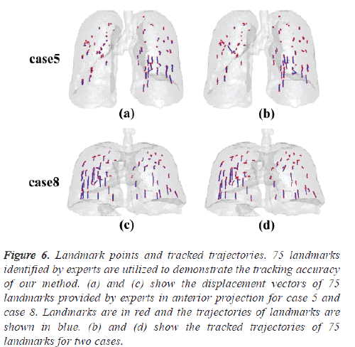
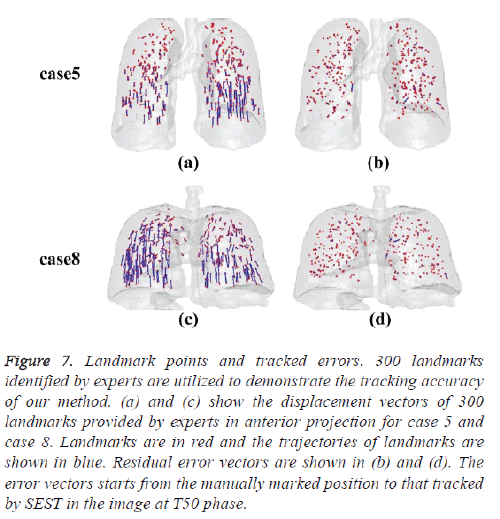
Figure 6 shows the isosurface rendering of the T00 lung images of case 5 and case 8. The trajectories of 75 landmarks from their T00 to T50 positions are displayed in the lung images also. The displacement vectors of 75 landmarks identified by experts for case 5 and case 8 are shown in figures 6a and 6c respectively, and the corresponding trajectories estimated by our method are shown in figures 6b and 6d respectively. Visually, most landmarks are tracked correctly. Noted that isolated landmarks are mistracked for case 5, figure 7 shows the displacement vectors and residual error vectors of 300 landmarks for case 5 and case 8. Figures 7a and 7c show the displacement vectors of 300 landmarks at T50 phase provided by experts in anterior projection for case 5 and case 8 respectively. Figures 7b and 7d show the corresponding residual error vectors. The error vectors starts from the manually marked position to that tracked by SEST in the image. Noted that these residual error vectors are short and distribute uniformly approximately. Several large error vectors can be observed which correspond with mistracking.
Figure 6: Landmark points and tracked trajectories. 75 landmarks identified by experts are utilized to demonstrate the tracking accuracy of our method. (a) and (c) show the displacement vectors of 75 landmarks provided by experts in anterior projection for case 5 and case 8. Landmarks are in red and the trajectories of landmarks are shown in blue. (b) and (d) show the tracked trajectories of 75 landmarks for two cases.
Figure 7: Landmark points and tracked errors. 300 landmarks identified by experts are utilized to demonstrate the tracking accuracy of our method. (a) and (c) show the displacement vectors of 300 landmarks provided by experts in anterior projection for case 5 and case 8. Landmarks are in red and the trajectories of landmarks are shown in blue. Residual error vectors are shown in (b) and (d). The error vectors starts from the manually marked position to that tracked by SEST in the image at T50 phase.
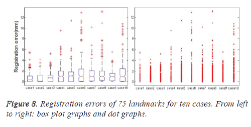
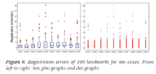
The box plots and the dot graph of the 75 and 300 landmarks registration errors of each case in the DIR-lab dataset are shown in figures 8 and 9 respectively. The number of outliers of the 75 landmarks target registration errors in all phases of each case is between 5 and 24, as listed in table 7. The average ratio of the 75 landmark points’ target registration error outliers is 2.8%. The number of the 300 landmark points’ target registration error outliers in the ME phase of each case is between 1 and 34. The average ratio of the 300 landmark points’ target registration error outliers is 2.7%. The outliers in Figure 8 and Figure 9 are caused by two reasons. The first one is that some of the landmarks are difficult to be tracked, which may create relative large tracking errors. The second one is that several landmarks marked by experts are not correct, which leads to deviation of the mean tracking error.
| cases | 75 landmarks | 300 landmarks | ||||
|---|---|---|---|---|---|---|
| number | mean | percent | number | mean | percent | |
| 1 | 24 | 3.1 | 6.4% | 34 | 3.5 | 11% |
| 2 | 7 | 3.5 | 1.8% | 1 | 2.9 | 0.3% |
| 3 | 5 | 3.7 | 1.3% | 4 | 4.4 | 1.3% |
| 4 | 8 | 6.3 | 2.1% | 6 | 8.6 | 2.0% |
| 5 | 5 | 6.6 | 1.3% | 5 | 11 | 1.7% |
| 6 | 12 | 9.7 | 3.2% | 5 | 7.9 | 1.7% |
| 7 | 7 | 6.3 | 1.8% | 4 | 5.8 | 1.3% |
| 8 | 15 | 7.5 | 4.0% | 7 | 8.3 | 2.3% |
| 9 | 5 | 4.2 | 1.3% | 11 | 3.5 | 3.7% |
| 10 | 19 | 8.9 | 2.4% | 6 | 8.1 | 2.0% |
Table 7: Comparison of the mean and standard deviation of tracking errors for the 75 and 300 landmarks before and after optimization.
Temporal smoothness
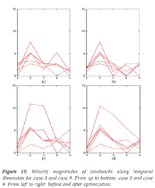
Furthermore, we will evaluate the temporal smoothness of the trajectories of landmarks after optimization. Case 8 and case 9 are selected as examples, where the tracking errors are improved greatly after optimization for case 8, and are almost fixed after optimization for case 9, especially in phase 4. The velocity magnitudes between consecutive phases for some trajectories in case 8 before and after optimization are illustrated in figures 10a and 10b respectively. Figure 10c and 10d show the results for case 9.
Based on the gradient of the velocity magnitudes, we select landmarks that change the velocity magnitudes significantly after optimization to plot. It can be observed that the velocity magnitudes are more stable after optimization for case 8 and case 9, which implies that smooth trajectories of landmarks can be achieved using our method.
Conclusion
4D-CT image registration algorithm based on local-global landmarks tracking is proposed in this paper. Spatial information is introduced into structure tensor to improve its description ability about image objects. The tracking algorithm based on the spatially extended structure tensor is capable of tracking landmarks position locally at all phases in the 4D-CT image. During the tracking procedure, the prior knowledge of respiratory motion can be used to limit the searching area. Furthermore, the spatial-temporal optimization model combining the image similarity, bending energy of transformations, and smoothness of landmark trajectories is a global tracking model to update the locally tracked results of landmarks. After optimization, the tracking errors of landmarks are decreased and the trajectories of landmarks are smoother. Experimental results of open source data from DIR-lab show that the local-global landmark tracking is feasible and robust.
